Meet Edith: Hybrid census in Burkina Faso: Bottom-up population modelling

Edith Darin

Introduction

In February 2020, the Institut National de la Statistique et de la Démographie du Burkina Faso (INSD) completed a census exercise aiming at enumerating the entire country population. Due to security issues in the North and the East regions, some communes (Burkinabe administrative unit level 3) could be only partially covered by governmental surveyors (38 out of 351 communes). The INSD requested support from the GRID3 (Geo-Referenced Infrastructure and Demographic Data for Development) project to estimate the unsurveyed population.

In December 2020, the INSD released its provisional census population counts for every communes which consisted in estimates for the unsurveyed areas, and census count corrected via a post-enumeration survey for the surveyed areas (Institut National de la Statistique et de la Démographie 2020). Parallel to that traditional publication, the INSD released also a high-resolution gridded population estimates, and its breakdown by age and sex group (WorldPop and Institut National de la Statistique et de la Démographie du Burkina Faso 2021).

The purpose of this methodological document is to explain:

The bottom-up modelling used to estimate population totals in incomplete communes
The top-down modelling used to disaggregate the published census population totals — a combination of estimation-based and enumeration-based commune totals — into high resolution gridded estimates

The produced dataset (WorldPop and Institut National de la Statistique et de la Démographie du Burkina Faso. 2021) can be downloaded from the WorldPop Open Population Repository (https://wopr.worldpop.org/?BFA/Population/v1.0) and explored on the woprVision data exploration interface (https://apps.worldpop.org/woprVision/).

Estimating Missed Communes

Model Method

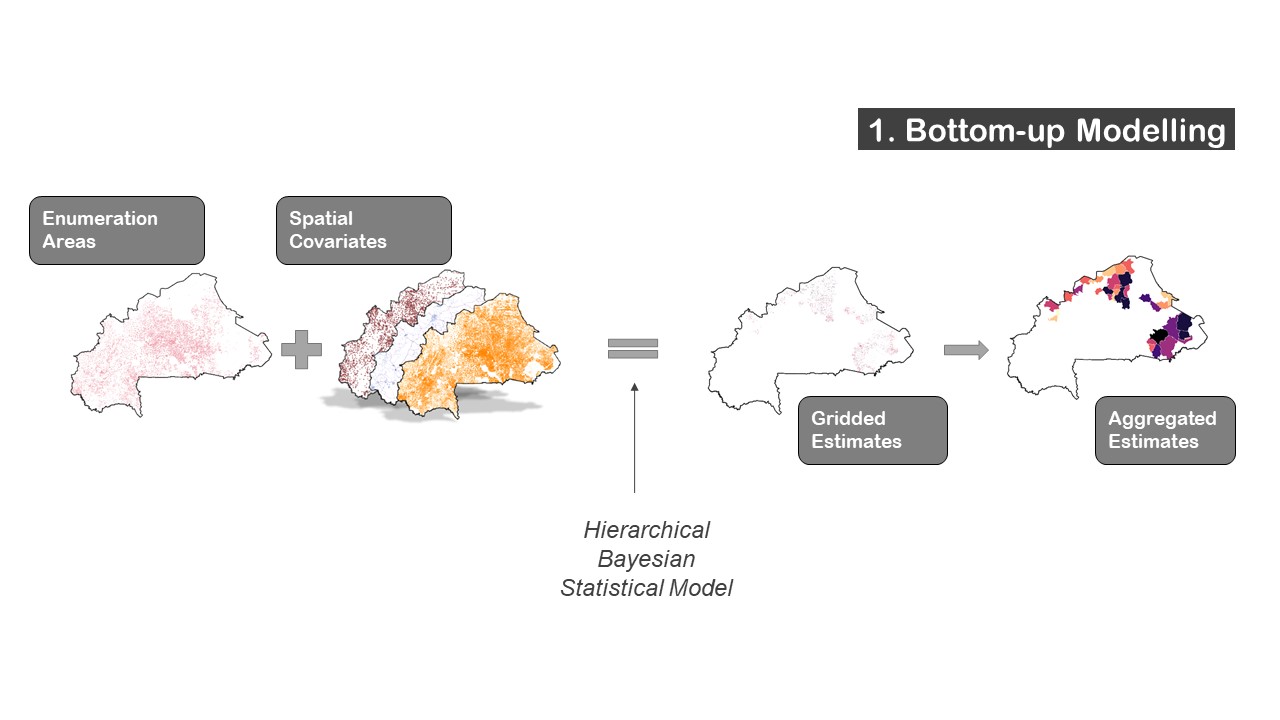
Figure 1: Schema for estimating population in missing communes

The ‘Bottom-up’ modelling followed the hierarchical Bayesian framework developed by Leasure et al. (2020) estimating population totals using sparse survey data. The method combines geospatial covariates available for the entire region of study with observed population data available only for a set of small-size clusters. The estimated relationship is then applied to the grid cells (3 arc-seconds, approximately 100m at the equator) of the unsurveyed areas to predict the population totals. To ensure consistency with the INSD traditional reporting, the gridded estimates were then aggregated at the commune level.

The hierarchical probabilistic framework enables to leverage statistical relationships between population and geospatial covariates from similar settled locations in order to predict elsewhere and to account for uncertainty in this process. The following equations describe the building blocks of the model:

\[ \begin{gathered} N_i \sim Poisson( D_i A_i ) \\ D_i \sim LogNormal( \bar{D}_i, \sigma_{l_1,l_2, l_3}) \\ \bar{D}_i = \alpha_{l_1,l_2, l_3} + \sum_{k=1}^{K} \beta_k x_{i,k} \\ \\ \alpha_{l_1,l_2, l_3} \sim Normal(11,3)\\ \beta_k \sim Normal(0,1)\\ \sigma_{l_1,l_2, l_3} \sim Truncated Normal(0,1,0) \end{gathered} \] with:

a Poisson distribution to model population count $N_i$ in enumeration area $i$
a lognormal distribution to model population density ($D_i$, which is the number of people per settled area in m$^2$, $A_i$)
a hierarchical setting for the variance of the lognormal, $\sigma$ estimated per level $l_1, l_2$ and $l_3$
a mean of the lognormal, $\bar{D}$ defined deterministically with a hierarchical slope $\alpha_{l_1,l_2,l_3}$, plus a set of $K$ covariates $x_k$ with related coefficients $\beta_k$

Model Implementation

Input data

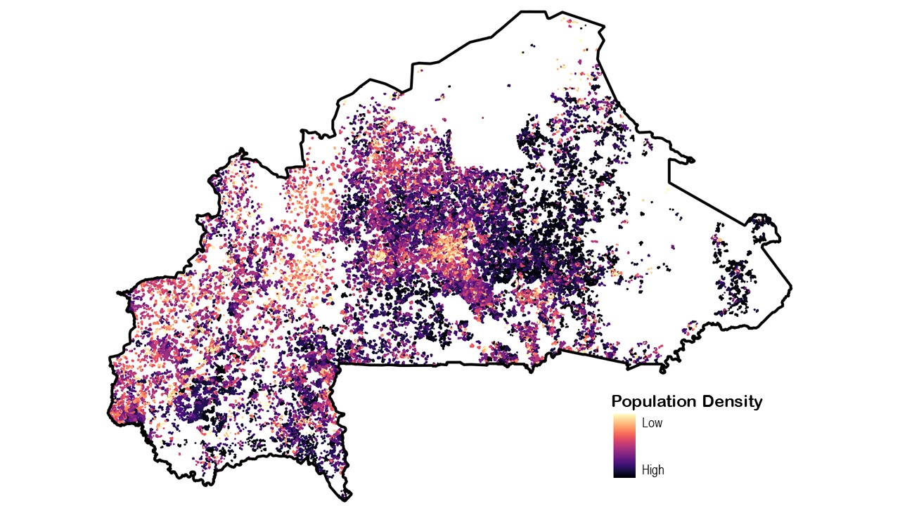
Figure 2: Population density of the selected enumeration areas

Population

The raw census database consists of the available GPS records for individual and collective resident households. At the time of the analysis, digital Enumeration Areas (EA) were not available, thus for modelling purposes, we compute ad hoc EA boundaries as envelopes around the GPS points belonging to the same enumeration area. A careful selection is then made to remove inaccurate EAs due to error in data collection, EA miss-attribution, imprecise GPS location or inaccurate GPS recording (due to the location where the surveyor entered the observation in the device). We implemented the criteria using quantitative metrics such as: the standard deviation of GPS points for each EA, the number of observations falling in one grid cell, the people/building ratio and the people/settled area ratio.

The final database used for modelling contains 15 817 EAs which represents 69% of the raw database.

To prevent overestimating population in unsurveyed communes, we removed from every EAs individuals that were recorded as migrants and originated from the unsurveyed communes. This provides us with a baseline population where displacement from the insecure communes is temporary ignored and tackled at a later stage.

Building footprints

A core covariate in our model is the building footprints layer provided by Ecopia.AI and Maxar Technologies (2019). It is a satellite-imagery-based features extraction at 5m and gives a precise estimate of the built-up area in Burkina Faso. Figure 3 illustrates this for an area in Ouagadougou.

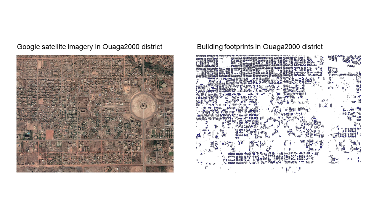
Figure 3: Example of the building footprints in Ouagadougou

From the building footprints we can calculate the settled area of each EA (i.e. the sum of each building area). During the model fitting, this is used to calculate population densities (people per settled area) from the observed counts.

The building footprints layer also provides the subset of grid cells for which to predict population count. We predict population only for the grid cells considered as settled, that contains at least one building from the building footprints layer.

Geospatial covariates

To study Burkina Faso spatial population distribution, we selected 5 covariates from different sources based on their assumed correlation to population densities and on shared range of values between the EA level dataset and the grid cell level dataset.

The final set of covariates is:

the count of buildings in a 5km buffer derived from the building footprints layer (Ecopia.AI and Maxar Technologies 2019)
the distance to temporary rivers and secondary roads provided in the Base Nationale de Données Topographiques (Institut Géographique du Burkina Faso 2015)
the friction surface used for the Access to Cities project (Weiss, Nelson, Gibson, Temperley, Peedell, Lieber, Hancher, Poyart, Belchior, Fullman, and others 2018a)
the UN-adjusted unconstrained gridded estimates from WorldPop that disaggregated the Burkina Faso 2019 census projections (WorldPop Research Group, University of Southampton et al. 2018)

For classifying settlement consistenly with census definition, we used the labelling of each EA in the census database as urban or rural to produce a settlement type prediction at grid cell level.

More precisely, we used the caret R package (Kuhn et al. 2020) to fit a Gradient Boosting Machine with two covariates, distance to high urban settlement (Institut Géographique du Burkina Faso 2015) and building count in a 500m window (Ecopia.AI and Maxar Technologies 2019). The area under the curve metric of the classification model is 0.98, indicating an almost perfect fit.

Model results

Implementing the model

The final models is composed of three nested levels for modelling population density: the modelled settlement type, the regions (Burkinabe administrative unit level 1) and the communes.

Model fit was done using the Stan software (Carpenter et al. 2017). Implementing scripts and distribution of estimated parameters can be found on Github: https://github.com/wpgp/BFA_population_v1_0_methods/tree/main/supplements.

To provide population totals for the unsurveyed communes, we aggregated the gridded bottom-up estimates using official boundaries (Institut Géographique du Burkina Faso 2015). Finally the estimated population totals were corrected for displacement based on the observed census migration status data. We added the migrants that were discarded when processing the census individual database (cf. Section ??) to the commune where they were enumerated and removed them from the unsurveyed commune where they were migrated from.

The model fit and prediction were done in R version 3.5.1., using the package rstan (Stan Development Team 2020), sf (Pebesma et al. 2020), raster (Hijmans et al. 2020), dplyr (Wickham et al. 2020), data.table (Dowle et al. 2020) and doParallel (Wallig et al. 2020).

Assessing the model goodness-of-fit

Prediction power of the final model is first assessed using a training dataset (70%) to fit the model and a test dataset (30%) to estimate the goodness-of-fit. The correlation between predictions and observations is 0.8. 95% of the test observations are in their 95% confidence interval. Bias (mean of residuals) is 45 people, imprecision (standard deviation of residuals) is 263 people and inaccuracy (mean of absolute residuals) is 169.

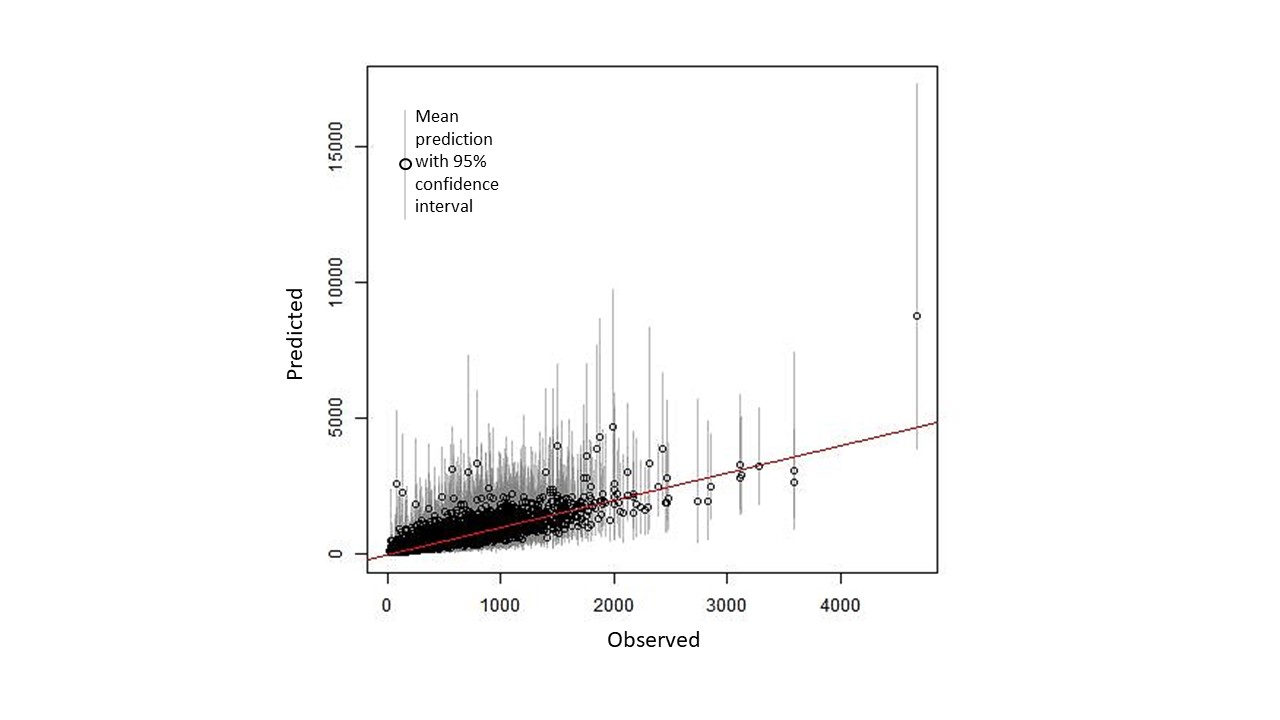
Figure 4: Scatterplot of observed vs. predicted population count on test EAs. Red line shows perfect prediction

The second assessment was undertaken on the population totals for the completed communes, totals that were corrected with omission rates from the post-enumeration survey. This reference data enables us to test the sensitivity of the estimates to the selection process, more precisely two crucial steps:

Drawing EA boundaries around GPS points. We have tested two alternative scenarios:
1. using a 25m buffer around the GPS points in Ouagadougou, a 25 m buffer in Saaba et Bobo-Dioulasso and a 100m buffer in the remaining zones;
2. using a 20m buffer around the GPS points in Ouagadougou, a 25m buffer in Bobo-Dioulasso and Saaba, a 80m buffer in other urban areas and a 120m buffer in rural areas.

Selecting the threshold used to discard EA based on the population density. We have tested two alternative options:
1. fixed national threshold and
2. custom thresholds based on the maximum population density per admin 2.

To assess the predicted totals, we compute a targeted Root Mean Squared Error for the complete communes nested in incomplete region:

\[ \sqrt[][\frac{1}{n} \sum_i (\hat{y}_i - y_i)^2] \]

where $n$ is the number of complete communes in incomplete regions ($n$=141), $y_i$ the observed census population totals for commune $i$ and $\hat{y}_i$ the predicted population totals for commune $i$.

Table 1: Sensitivity analysis results on predicted totals
Selection procedures		EA (%)^*	RMSE^†
Delineation	Density threshold
Scenario 1	0.16	5	12 163
Scenario 2	0.16	4	10 871
Scenario 2	0.9 x maximum	7	9 966
Scenario 2	0.8 x maximum	9	9 745
^* Additional EAs discarded because of selection procedures (in percentage)
^† RMSE was compiled over the complete communes from incomplete regions

Table 1 shows that differentiating the size of the buffer between urban types does improve the goodness-of-fit. Furthermore choosing a resident density threshold based on the admin 2 maximum resident density succeeds in giving a more representative EA dataset that increase the external goodness-of-fit. Final model is represented in bold.

Estimating Gridded Population for the Entire Country

Model Method

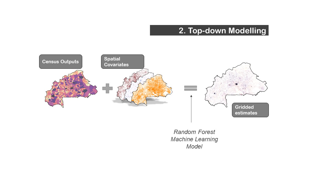
Figure 5: Schema for estimating gridded population for the entire country

To disaggregate the released communes census count into high-resolution gridded estimates, we adapted the dasymetric mapping explained in Stevens and al. (2015b) using the openly accessible scripts written by Bondarenko and al. (2018). The method consists in modeling population density by combining geospatial and remotely-sensed data in a Random Forest framework. This framework is chosen for its great predictive performance, the absence of complicated tuning parameter and its robustness to multicolinearity and multi-scale issues in the predictors (Robnik-Šikonja 2004).

Once the model is fitted at administrative level, it is then applied to each grid cell to obtain prediction of population density at a 100m x 100m resolution. This predicted density is then used as a weighting layer to disaggregate census population counts into the settled pixels based on a building footprint dataset from Ecopia.AI and Maxar Technologies (2019). The census counts are thus unevenly distributed across space to better reflect heterogeneous human settlement patterns.

Model Implementation

Input data

Population

The officially released population counts at commune level, displayed in Figure 6 combine the surveyed totals (adjusted with post-enumeration survey non-respondent rates) and the estimated bottom-up totals.

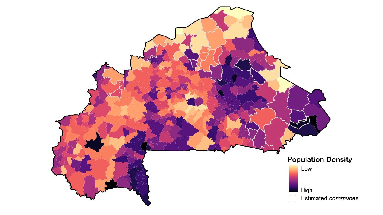
Figure 6: Map of commune population totals

The census provisional results include also an age and sex decomposition in 18 five-years-groups at national level (Institut National de la Statistique et de la Démographie 2020). These will be used to create the age and sex rasters.

Building footprints

The building footprints layer was already presented in Section ??. For the disagregation exercise we derived four building attributes in addition to building count and settled grid cells, namely:

Building area
Building perimeter
Nearest neighbour distance
Nearest neighbour proximity (1/distance)

The above building attributes are summarised at grid cell level using eight aggregation methods: mean, median (med), standard deviation (sd), mean absolute deviation (mad), minimum, maximum, relative standard deviation (mean/sd) and relative mad (mad/med). Metrics based on the standard deviation or mean absolute deviation indicate the level of heterogeneity of the pixel.

Despite the seemingly similarities between some building-footprints derived covariates, the underlying goal is to increase weak signals for the Random Forest modelling whose predictions will not be impacted by high level correlation (Genuer, Poggi, and Tuleau-Malot 2010).

Geospatial covariates

In addition to spatial settlement characteristics (contained in the building footprints), we use geospatial covariates to explain the broader context of population distribution.

We constructed 27 additional covariates from six data sources:

3 from the covariates mapped by the Malaria Atlas Project for their ‘Accessibility to cities’ and ‘Housing in Africa’ projects: travel time in 2015, friction surface in 2015 (Weiss, Nelson, Gibson, Temperley, Peedell, Lieber, Hancher, Poyart, Belchior, Fullman, and others 2018b) and mapping of improved housing conditions in 2015 (Tusting et al. 2019).
4 from the climatic covariates from the Climatic Research Unit: temperature, precipitation, cloud cover and wetness (Harris et al. 2020)
9 from the ESACCI land cover classification (Buchhorn et al. 2020), divided in the 9 overarching classes for which we computed the grid-cell-based distance
3 from the settlement extent (Center for International Earth Science Information Network and Novel-T 2020) classified in 3 types (hamlet, small settlement, built-up areas) for which we computed the grid-cell-based distance
5 from the Base Nationale de Données Topographiques (Institut Géographique du Burkina Faso 2015): the rivers network, the roads network and the settlement points classified in three types according to their urban status (low, middle, high), for which we computed the grid-cell-based distance
the WorldPop gridded census projection of 2019 (WorldPop Research Group, University of Southampton et al. 2018)

Model Results

Implementing the model

To model the relationship between census data and the entire set of covariates, we transform the population count into population density by dividing it with the area of all settled grid cells in the commune and then log-transform it (Forrest R. Stevens et al. 2015a). We then average the covariates using zonal mean for every communes. The procedure developed in Bondarenko et al. (2018) was used to both tune the Random Forest model and select covariates using their importance score to speed up the per-pixel prediction.

Once the model is fitted at commune level, we use it to predict the population density for each grid cell. This predicted density is then used as a weight to disaggregate the total population count for each commune. The disaggregated gridded population estimates are multiplied by the age and sex proportions from the national demographic pyramid to estimate population counts per age and sex group for each grid cell.

The code for the model fit and prediction can be found on Github: https://github.com/wpgp/BFA_population_v1_0_methods

The fit and the prediction were done in R version 3.5.1., using the package randomForest (Cutler and Wiener 2018), sf_0.9-5 (Pebesma et al. 2020), raster (Hijmans et al. 2020), dplyr (Wickham et al. 2020), data.table (Dowle et al. 2020) and doParallel (Wallig et al. 2020).

Assessing the model goodness-of-fit

Covariates importance We assess the importance of a predictor by showing the relative increase in the mean square error when the predictor is removed from the model. The order of magnitude might not be robust to the collinearity observed in the covariates set but the relative ranking is (Genuer, Poggi, and Tuleau-Malot 2010).

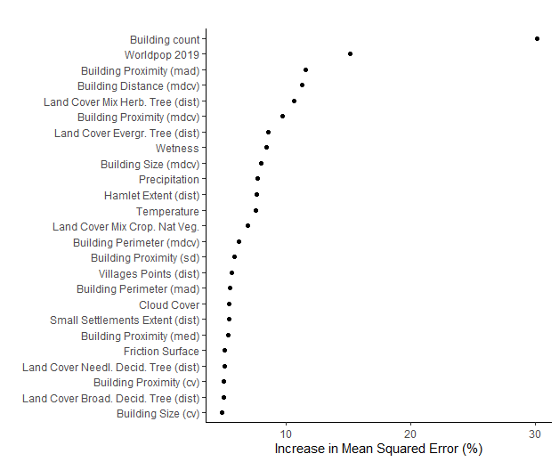
Figure 7: Top 25 Covariates importance in the Random Forest model

Figure 7 shows that the mean building count per pixel is by far the most important predictor, followed by the gridded population projections from WorldPop that informs population distribution from previous censuses. The presence in the top 25 covariates of different land cover classes confirms previous findings on the predictive power of land classification (Lloyd et al. 2019).

An interesting additional feature is the strong predictive power of building-derived metric depicting heterogeneity in a grid cell (standard deviation -sd-, mean absolute deviation -mad-, coefficient of variation -cv- and relative mean absolute deviation -mdcv-).

Assessing the model A metric that is commonly used to assess a Random Forest model is the percentage of variance explained (Liaw and Wiener 2002). It corresponds to the “out-of-bag” mean squared error divided by the variance of the observations: \[1 - \frac{\sum_i (y_i - \hat{y}_i)^2}{\sum_i (y_i - \bar{y})^2}\]whre $y_i$ is the observed population totals for commune $i$ with $\bar{y}$ its corresponding average and $\hat{y}_i$ is the predicted population totals for commune $i$ on a test dataset.

In our model the percentage of variance explained is equal to 70.1%. For comparison the model developed by Stevens et al. (2015b) for Burkina Faso using census projections and a standardised set of covariates (Lloyd et al. 2019) had a percentage of variance explained of 59.1%¹.

The difference is explained by the custom set of covariates used in our model, especially the one derived from the building footprints, and the restriction of population estimation and prediction to the settled grid cells.

Assessing the prediction In Stevens and al. (2015b) external validation was undertaken by applying the modelling process to a coarser census scale and then aggregating predicted population per pixel at the finer census unit to compare it with census results. However in Burkina Faso, the coarser administrative unit after the commune is the province level that has only 45 units. We considered this sample size too small to perform a meaningful model assessment of the Random Forest modelling.

Nonetheless, we had access to the raw census database where household GPS points provide a geo-tagging of enumeration areas across the country. Thus, this oﬀers the possibility to check the model performance at a fine spatial scale. We manually selected a subset of 50 enumeration areas across the country in diﬀerent settlement settings based on the visual assessment of the satellite imagery. We then computed a predicted population by summing up the corresponding grid cells and performed a comparison analysis based on the relative prediction error (Figure 8 and 9):

\[ \frac{\hat{y} - y}{y}*100 \]

where $\hat{y}$ is the predicted and $y$ the observed EA population count.

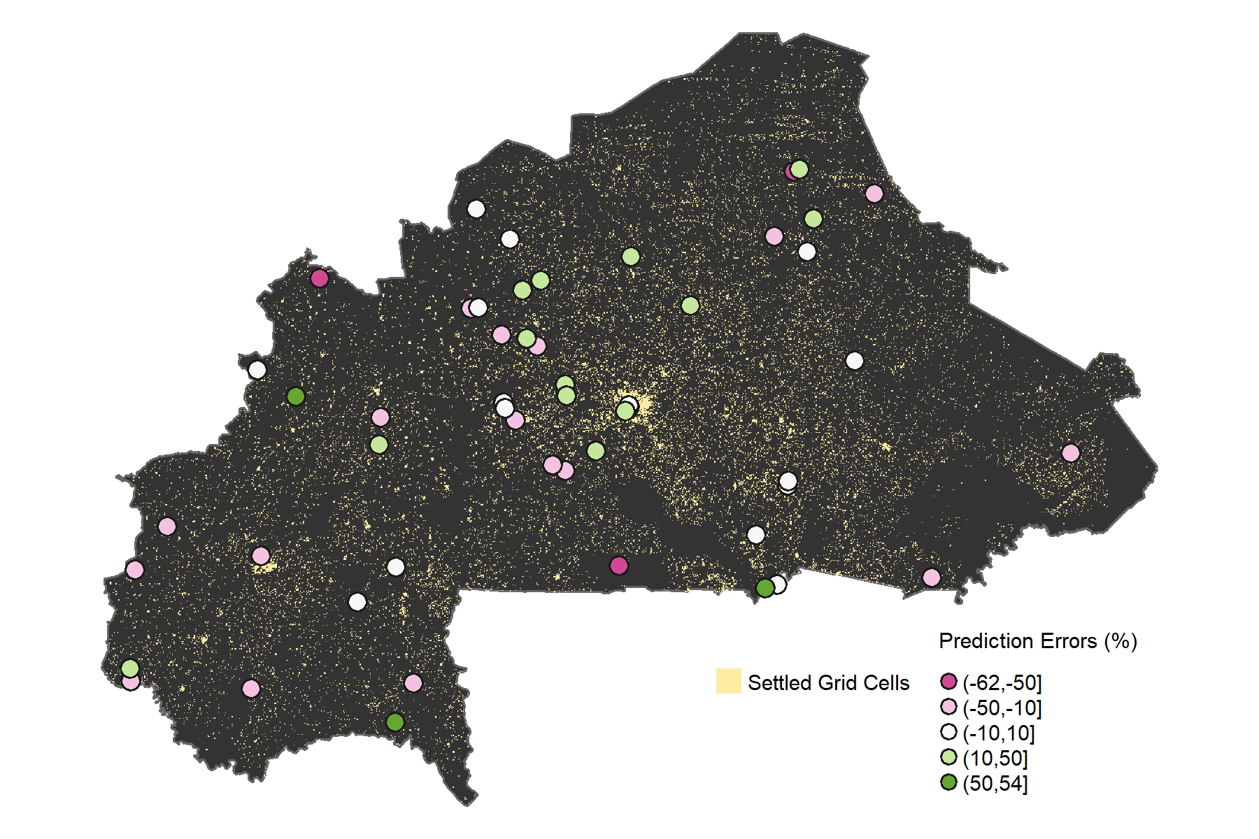
Spatial distribution of the relative prediction errors. Dots shows the location of the selected EAs. The colours show the ranges of predictive errors. Settled pixels are shown in yellow.

Figure 8: Spatial distribution of the relative prediction errors. Dots shows the location of the selected EAs. The colours show the ranges of predictive errors. Settled pixels are shown in yellow.

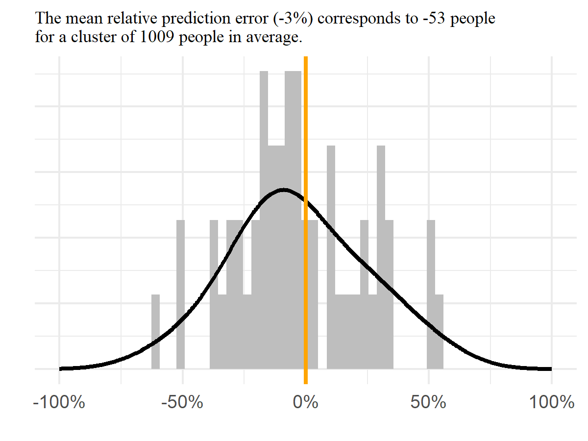
$Distribution of the relative prediction errors.Grey bars represent each of the 50 selected EAs.The orange line shows the location of the 0\% error, the black line summarises the overall error distribution.$

Figure 9: Distribution of the relative prediction errors.Grey bars represent each of the 50 selected EAs.The orange line shows the location of the 0% error, the black line summarises the overall error distribution.

Figure 9 shows an average bias of the prediction of -3%. Imprecision (std. of relative error) is 27% and inaccuracy 21% (mean of the absolute relative error).

The greater prediction errors are occurring in rural area as shown by the spatial distribution of the settled cells without clear geographical clustering (Figure 8).

Discussion

The assumptions and limitations of this study can be summarised by topics.

Country extent Administrative boundary datasets include the entire surface of the country. Any settled grid cells outside of the boundaries from the Base Nationale de Données Topographiques (Institut Géographique du Burkina Faso 2015) were not included.

Data date Although the input data have varying reference years, the estimates should be considered as representing late 2019 as thisis the date of the census data collection.

Settlement type The population counts in areas with primarily non-residential buildings may be over-estimated. Caution should be taken when using the population data in industrial (and other primarily non-residential) areas. Furthermore little variation can be modelled for densely populated urban areas. This is due to the scale of the input data used to fit the model, namely at administrative level 3, that does not capture well variation in a dense city such as Ouagadougou. Therefore precautions shall be taken when focusing the analysis in urban zones.

Building footprints We assume that the building footprints data is accurate and that each building polygon corresponds to a building structure. However the date of the satellite imagery spans from 2009 to 2019 (see Figure 10). The estimated population counts may be inaccurate in areas where the imagery is old and buildings have recently been constructed. This issue was observed in the towns of Zorgho, Bâtié and Nanoro. But it is minimized by old satellite imagery being only used in remote area.

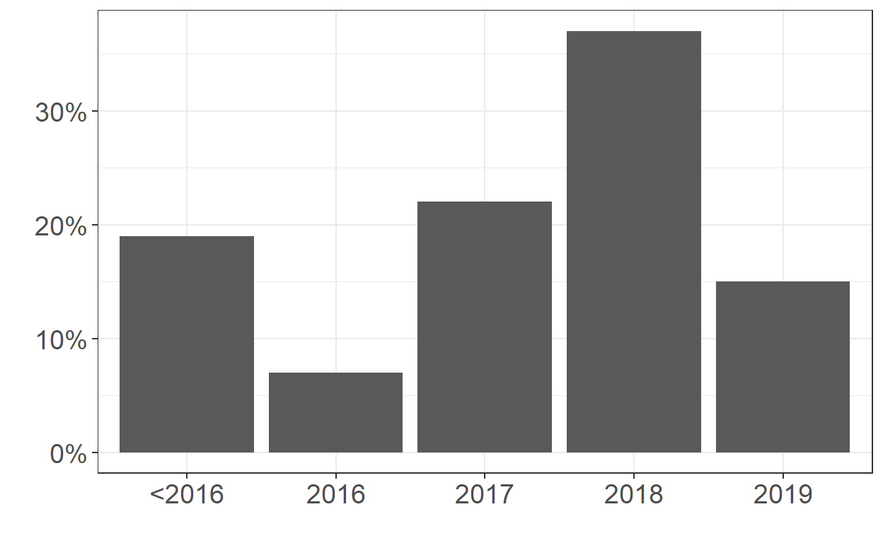
Figure 10: Satellite imagery date used for extracting building footprints by Ecopia.AI, and Maxar Technologies. (2019)

Discrete population pattern Administrative boundaries are visible in the disagregated estimates whereby sharp population differences can be found for neighboring grid cells along the administrative unit delimitation. This is the consequence of the dasymetric top-down disagregation which ensures that the sum of every grid cells of the administrative unit does match with the total provided.

Modeled population The population that is predicted is the de jure resident population as defined by the INSD, that is planning in staying or having stayed already six months at the place where the census is taking place. This population dataset represent neither the ambient population, nor captures internal migration below the commune level.

Age and sex pyramid The age and sex proportions are released by the INSD at the national level, therefore no subnational variations in proportion were considered for the gridded estimates.

Contributions

This work is part of the GRID3 (Geo-Referenced Infrastructure and Demographic Data for Development) project funded by the Bill and Melinda Gates Foundation (BMGF) and the United Kingdom’s Department for International Development (OPP1182408). Project partners include WorldPop at the University of Southampton, the United Nations Population Fund (UNFPA), Center for International Earth Science Information Network (CIESIN) in the Earth Institute at Columbia University, and the Flowminder Foundation. The Institut National de la Statistique et de la Démographie supported, facilitated this work, reviewed the results and provided the census database. The modelling work, geospatial data processing, stakeholder engagement and model report was led by Edith Darin with help from Mathias Kuépié. Support for the statistical modelling was provided by Gianluca Boo, Claire A. Dooley, Douglas R. Leasure and Chris W. Jochem. Gianluca Boo, Douglas R. Leasure and Attila N. Lazar provided a thorough review of the manuscript. Oversight was done by Andrew J. Tatem and Attila N. Lazar.

License

This report may be redistributed using a Creative Commons Attribution 4.0 International (CC BY 4.0) License.

Suggested Citation

WorldPop and Institut National de la Statistique et de la Démographie du Burkina Faso. 2021. Census-based gridded population estimates for Burkina Faso (2019), version 1.0. WorldPop, University of Southampton. doi:10.5258/SOTON/WP00687.

References

Bondarenko, Maksym, Jeremiah Nieves, Alessandro Sorichetta, Forrest R Stevens, Andrea E Gaughan, Andrew Tatem, and others. 2018. “wpgpRFPMS: WorldPop Random Forests Population Modelling r Scripts, Version 0.1. 0.”

Buchhorn, Marcel, Bruno Smets, Luc Bertels, Bert De Roo, Myroslava Lesiv, Nandin-Erdene Tsendbazar, Martin Herold, and Steffen Fritz. 2020. “Copernicus Global Land Service: Land Cover 100m: collection 3: epoch 2019: Globe.” Zenodo. https://doi.org/10.5281/zenodo.3939050.

Carpenter, Bob, Andrew Gelman, Matthew D Hoffman, Daniel Lee, Ben Goodrich, Michael Betancourt, Marcus Brubaker, Jiqiang Guo, Peter Li, and Allen Riddell. 2017. “Stan: A Probabilistic Programming Language.” Journal of Statistical Software 76 (1). https://doi.org/10.18637/jss.v076.i01.

Center for International Earth Science Information Network, and Novel-T. 2020. “Grid3 Burkina Faso Settlement Extents Version 01, Alpha.” https://doi.org/10.7916/d8-h47k-8637.

Cutler, Fortran original by Leo Breiman and Adele, and R. port by Andy Liaw and Matthew Wiener. 2018. randomForest: Breiman and Cutler’s Random Forests for Classification and Regression. https://CRAN.R-project.org/package=randomForest.

Dowle, Matt, Arun Srinivasan, Jan Gorecki, Michael Chirico, Pasha Stetsenko, Tom Short, Steve Lianoglou, et al. 2020. Data.table: Extension of ’Data.frame’. https://CRAN.R-project.org/package=data.table.

Ecopia.AI, and Maxar Technologies. 2019. Digitize Africa Data.

Genuer, Robin, Jean-Michel Poggi, and Christine Tuleau-Malot. 2010. “Variable Selection Using Random Forests.” Pattern Recognition Letters 31 (14): 2225–36.

Harris, Ian, Timothy J Osborn, Phil Jones, and David Lister. 2020. “Version 4 of the CRU TS Monthly High-Resolution Gridded Multivariate Climate Dataset.” Scientific Data 7 (1): 1–18.

Hijmans, Robert J., Jacob van Etten, Michael Sumner, Joe Cheng, Dan Baston, Andrew Bevan, Roger Bivand, et al. 2020. Raster: Geographic Data Analysis and Modeling. https://CRAN.R-project.org/package=raster.

Institut Géographique du Burkina Faso. 2015. “Base Nationale de Données Topographiques.”

Institut National de la Statistique et de la Démographie. 2020. “Cinquième Recensement Général de la Population et de l’Habitation du Burkina Faso - Résultats préliminaires.” INSD Ouagadougou, Burkina Faso.

Kuhn, Max, Jed Wing, Steve Weston, Andre Williams, Chris Keefer, Allan Engelhardt, Tony Cooper, et al. 2020. Caret: Classification and Regression Training. https://CRAN.R-project.org/package=caret.

Leasure, Douglas R, Warren C Jochem, Eric M Weber, Vincent Seaman, and Andrew J Tatem. 2020. “National Population Mapping from Sparse Survey Data: A Hierarchical Bayesian Modeling Framework to Account for Uncertainty.” Proceedings of the National Academy of Sciences.

Liaw, Andy, and Matthew Wiener. 2002. “Classification and Regression by randomForest.” R News 2 (3): 18–22. https://CRAN.R-project.org/doc/Rnews/.

Lloyd, Christopher T, Heather Chamberlain, David Kerr, Greg Yetman, Linda Pistolesi, Forrest R Stevens, Andrea E Gaughan, et al. 2019. “Global Spatio-Temporally Harmonised Datasets for Producing High-Resolution Gridded Population Distribution Datasets.” Big Earth Data 3 (2): 108–39. https://doi.org/10.1080/20964471.2019.1625151.

Pebesma, Edzer, Roger Bivand, Etienne Racine, Michael Sumner, Ian Cook, Tim Keitt, Robin Lovelace, et al. 2020. Sf: Simple Features for r. https://CRAN.R-project.org/package=sf.

Robnik-Šikonja, Marko. 2004. “Improving Random Forests.” In European Conference on Machine Learning, 359–70. Springer.

Stan Development Team. 2020. “RStan: The R Interface to Stan.” http://mc-stan.org/.

Stevens, Forrest R., Andrea E. Gaughan, Catherine Linard, and Andrew J. Tatem. 2015a. “Disaggregating Census Data for Population Mapping Using Random Forests with Remotely-Sensed and Ancillary Data.” PLOS ONE 10 (2): e0107042. https://doi.org/10.1371/journal.pone.0107042.

Stevens, Forrest R, Andrea E Gaughan, Catherine Linard, and Andrew J Tatem. 2015b. “Disaggregating Census Data for Population Mapping Using Random Forests with Remotely-Sensed and Ancillary Data.” PloS One 10 (2). https://doi.org/10.1371/journal.pone.0107042.

Tusting, Lucy S, Donal Bisanzio, Graham Alabaster, Ewan Cameron, Richard Cibulskis, Michael Davies, Seth Flaxman, et al. 2019. “Mapping Changes in Housing in Sub-Saharan Africa from 2000 to 2015.” Nature 568 (7752): 391–94.

Wallig, Michelle, Microsoft Corporation, Steve Weston, and Dan Tenenbaum. 2020. doParallel: Foreach Parallel Adaptor for the ’Parallel’ Package. https://CRAN.R-project.org/package=doParallel.

Weiss, D J, A Nelson, HS Gibson, W Temperley, S Peedell, A Lieber, M Hancher, E Poyart, S Belchior, N Fullman, and others. 2018b. “A Global Map of Travel Time to Cities to Assess Inequalities in Accessibility in 2015.” Nature 553 (7688): 333–36.

Weiss, D J, A Nelson, HS Gibson, W Temperley, S Peedell, A Lieber, M Hancher, E Poyart, S Belchior, N Fullman, and others. 2018a. “A Global Map of Travel Time to Cities to Assess Inequalities in Accessibility in 2015.” Nature 553 (7688): 333336.

Wickham, Hadley, Romain François, Lionel Henry, Kirill Müller, and RStudio. 2020. Dplyr: A Grammar of Data Manipulation. https://CRAN.R-project.org/package=dplyr.

WorldPop Research Group, University of Southampton, Department of Geography and Geosciences, University of Louisville, Departement de Geographie, Universite de Namur, and Center for International Earth Science Information Network (CIESIN), Columbia University. 2018. “Global High Resolution Population Denominators Project - Funded by the Bill and Melinda Gates Foundation (Opp1134076).” https://doi.org/10.5258/SOTON/WP00645.

WorldPop, and Institut National de la Statistique et de la Démographie du Burkina Faso. 2021. “Census-Based Gridded Population Estimates for Burkina Faso (2019), Version 1.0.” WorldPop, University of Southampton. https://doi.org/10.5258/SOTON/WP00687.

See Burkina Faso 2019 in http://dx.doi.org/10.5258/SOTON/WP00645 for more details.↩︎