SICSS-Covenant:Using gridded population to gain spatial insights in R

I have been invited to present at the Summer Institute for Computational Social Sciences in University of Covenant. My talks starts is about gridded population as a tool to link demographics and geography. It starts with a global overview of the definition, production and use of this innovative data and pursues with a hands-on in R to gain spatial insights on demography in Nigeria.

Extract from the github repo that contains the session’s material.

Linking demographics and geography: Using gridded population to gain spatial insights in R

Introduction

Access to high-resolution population counts is key for local, national and international decision-making and intervention. It supports data-driven planning of critical infrastructures, such as schools, health facilities and transportation networks.

WorldPop has developed modelling techniques to estimate population in grid cells of 100m by 100m by disaggregating census-based population totals for the entire world, leveraging the growing availability of products derived from satellite imagery. This level of detail offers the advantage of flexible aggregation of the population estimates within different administrative and functional units, for instance, school catchment areas and health zones.

This session will cover the notion of gridded population, a data format at the crossroad of demography and geography. We will then have a brief overview of openly available satellite-imagery-based products that can be used for modelling gridding population and beyond, such as settlement maps. Finally, we will have some hands-on to extract information from a gridded population covering the following R packages for geospatial analysis: sf (Pebesma, E., 2018), raster (Hijmans, R., 2021), and tmap (Tennekes, M., 2018).

Challenge

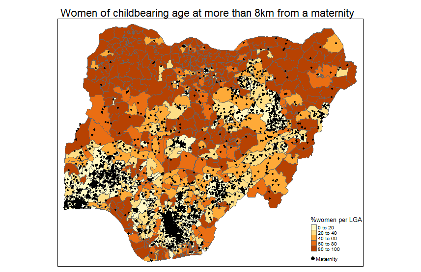
We will study the question: How many women of childbearing age are struggling to access maternal health services?

Concepts

This tutorial covers the concepts of:

• interactive mapping

• vector file reading and filtering

• raster file reading

• buffering

• rasterising

• zonal statistics

• masking

Contents

On github is stored the raw material for this tutorial. The script for_students.R contains the workflow with the questions. The script teaching.R contains the workflow with the answers. The powerpoint SICSS_20220624_griddedPop.pptx contains the presentation.

Data used

For that purpose, we will need to access three data sources:

1. Population data from the Bottom-up gridded population estimates for Nigeria, version 2.0, produced jointly by WorldPop and the National Population Commission of Nigeria and accessible here,

2. Health facilities locations produced by GRID3 Nigeria and accessible here,

3. Local Government Area operational boundaries released by GRID3 Nigeria and accessible here On github the three data file are stored for this tutorial.

## Practical

library(tidyverse) #R library to manipulate table data
library(tmap) # R library to plot interactive maps
library(kableExtra) # R library for nice tables

tmap_mode('view') # set tmap as interactive
tmap_options(check.and.fix = TRUE) 

Defining the study area ————————————————-

library(sf) # R library to manipulate spatial data

We load the vector file of administrative regions in Nigeria

lga <- st_read(
  paste0(
    data_path,
    '/GRID3_Nigeria_-_Local_Government_Area_Boundaries/GRID3_Nigeria_-_Local_Government_Area_Boundaries.shp'))

Reading layer `GRID3_Nigeria_-_Local_Government_Area_Boundaries' from data source `C:\Users\ecd1u18\Documents\SICSS-covenant-gridded-population\data\GRID3_Nigeria_-_Local_Government_Area_Boundaries\GRID3_Nigeria_-_Local_Government_Area_Boundaries.shp' 
  using driver `ESRI Shapefile'
Simple feature collection with 774 features and 7 fields
Geometry type: MULTIPOLYGON
Dimension:     XY
Bounding box:  xmin: 2.692613 ymin: 4.270204 xmax: 14.67797 ymax: 13.88571
Geodetic CRS:  WGS 84

lga %>% 
      glimpse()

Rows: 774
Columns: 8
$ OBJECTID   <int> 1, 2, 3, 4, 5, 6, 7, 8, 9, 10, 11, 12, 13, 14, 15~
$ lga_code   <chr> "10001", "10002", "10003", "10004", "10005", "100~
$ state_code <chr> "DE", "DE", "DE", "DE", "DE", "DE", "DE", "DE", "~
$ lga_name_x <chr> "Aniocha North", "Aniocha South", "Bomadi", "Buru~
$ mean       <dbl> 91927.45, 193913.27, 32604.42, 53159.27, 153016.5~
$ Shape__Are <dbl> 0.033182160, 0.070862318, 0.016922270, 0.14636025~
$ Shape__Len <dbl> 0.8457545, 1.2001197, 1.0004980, 2.4157890, 1.068~
$ geometry   <MULTIPOLYGON [°]> MULTIPOLYGON (((6.438156 6...., MULT~

We plot using tmap interactive functions

tm_shape(lga)+
  tm_polygons()

We will focus our analysis in the local government area of Ado Odo/Ota

lga_Ado <- lga %>% 
  filter(lga_name_x=='Ado Odo/Ota')


tm_shape(lga_Ado)+
  tm_borders(col='orange', lwd=5)+
  tm_shape(lga)+
  tm_borders()+
  tm_basemap('OpenStreetMap')

Discovering the health facilities dataset ——————————-

health_facilities <- st_read(
  paste0(
    data_path, 
    '/GRID3_Nigeria_-_Health_Care_Facilities_/GRID3_Nigeria_-_Health_Care_Facilities_.shp'))

Reading layer `GRID3_Nigeria_-_Health_Care_Facilities_' from data source `C:\Users\ecd1u18\Documents\SICSS-covenant-gridded-population\data\GRID3_Nigeria_-_Health_Care_Facilities_\GRID3_Nigeria_-_Health_Care_Facilities_.shp' 
  using driver `ESRI Shapefile'
Simple feature collection with 46146 features and 20 fields
Geometry type: POINT
Dimension:     XY
Bounding box:  xmin: 2.70779 ymin: 4.281802 xmax: 14.63638 ymax: 13.86524
Geodetic CRS:  WGS 84

health_facilities %>% 
  st_drop_geometry() %>% 
  glimpse()

Rows: 46,146
Columns: 20
$ FID        <int> 1, 2, 3, 4, 5, 6, 7, 8, 9, 10, 11, 12, 13, 14, 15~
$ editor     <chr> "tosin.williams", "mokobia.chidinma", "tosin.will~
$ timestamp  <date> 2020-07-04, 2020-07-04, 2020-07-04, 2020-07-04, ~
$ lga_code   <int> 124, 124, 124, 124, 124, 124, 124, 124, 124, 124,~
$ lga_name   <chr> "Maiduguri", "Maiduguri", "Maiduguri", "Maiduguri~
$ ward_name  <chr> "Maisandari", "Maisandari", "Maisandari", "Maisan~
$ ward_code  <chr> "12413", "12413", "12413", "12413", "12413", "124~
$ longitude  <dbl> 13.14832, 13.14718, 13.14227, 13.14134, 13.11913,~
$ latitude   <dbl> 11.82232, 11.82161, 11.79810, 11.81027, 11.83188,~
$ updated_on <chr> "2019-03-01", "2019-03-01", "2019-03-01", "2019-0~
$ accessibil <chr> NA, "Unknown", NA, NA, NA, "Unknown", "Unknown", ~
$ functional <chr> "Unknown", "Functional", "Functional", "Functiona~
$ category   <chr> "Primary Health Center", "Primary Health Center",~
$ ownership  <chr> "Private", "National Primary Healthcare Developme~
$ type       <chr> "Primary", "Primary", "Primary", "Primary", "Prim~
$ source     <chr> "eHA Polio", "Measles Campaign", "eHA Polio", "He~
$ alternate_ <chr> "Nursing Home", "Nursing Home", "Atla Medical Cen~
$ primary_na <chr> "G R A Nursing Home", "Gishili Health Center", "G~
$ globalid   <chr> "af719462-abfd-4f47-9dc3-0987164e75ac", "a29b0328~
$ state_code <chr> "BR", "BR", "BR", "BR", "BR", "BR", "BR", "BR", "~

health_facilities_Ado <- health_facilities %>% 
  filter(lga_name=='Ado Odo/Ota')

EXERCISE: How many health facilities in Ado Odo/Ota?

Click for the solution

dim(health_facilities_Ado)

[1] 216  21

We now represent the health facilities in Ado by facility types. We specify than on hoover the name of the facility primary_na is shown and on click the name, primary_na, the function status, functional and the source of the information, source.

tm_shape(health_facilities_Ado)+
  tm_dots(col='type', size=0.07, id='primary_na', 
          popup.vars=c('category','functional','source'))+
  tm_basemap('OpenStreetMap')+
  tm_shape(lga_Ado)+
  tm_borders(lwd=4)

EXERCISE: How many health facilities are offering tertiary services in Ado Odo/Ota?

Click for the solution

table(health_facilities_Ado$type)

  Primary Secondary  Tertiary 
      205         6         5 

Discovering the gridded population dataset ——————————

library(raster) # R library to manipulate raster data

pop <- raster(
  paste0(
    data_path, 
    '/NGA_population_v2_0_gridded/NGA_population_v2_0_gridded.tif'))

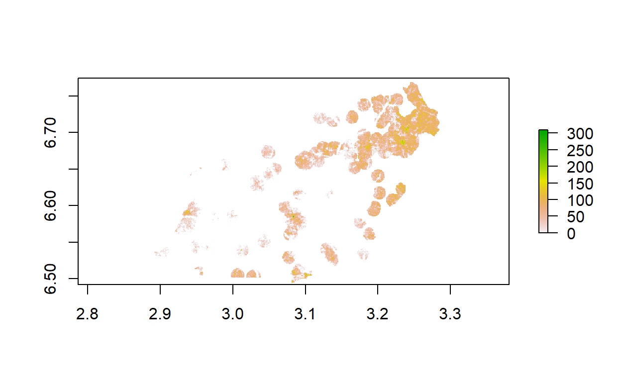
First spatial manipulation: cropping (or cutting a raster file to the extent of another spatial file, here the extent or bounding box of the Ado LGA)

pop_Ado <- crop(pop, lga_Ado)
plot(pop_Ado)

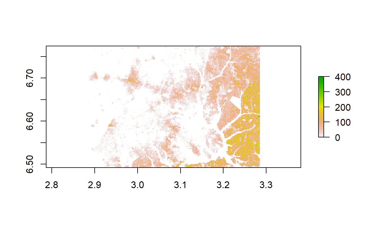
Second spatial manipulation: masking (or modifying the values of raster grid cells designated by a second raster, here the values outside of the boundaries of the Ado LGA )

pop_Ado <- mask(pop_Ado, lga_Ado)
plot(pop_Ado)

And now we combine health facilities informaiton with gridded population

tm_shape(health_facilities_Ado)+
  tm_dots(col='type', size=0.07, id='primary_na', 
          popup.vars=c('category','functional','source'))+
  tm_basemap('OpenStreetMap')+
  tm_shape(pop_Ado)+
  tm_raster()+
  tm_shape(lga_Ado)+
  tm_borders(lwd=4)

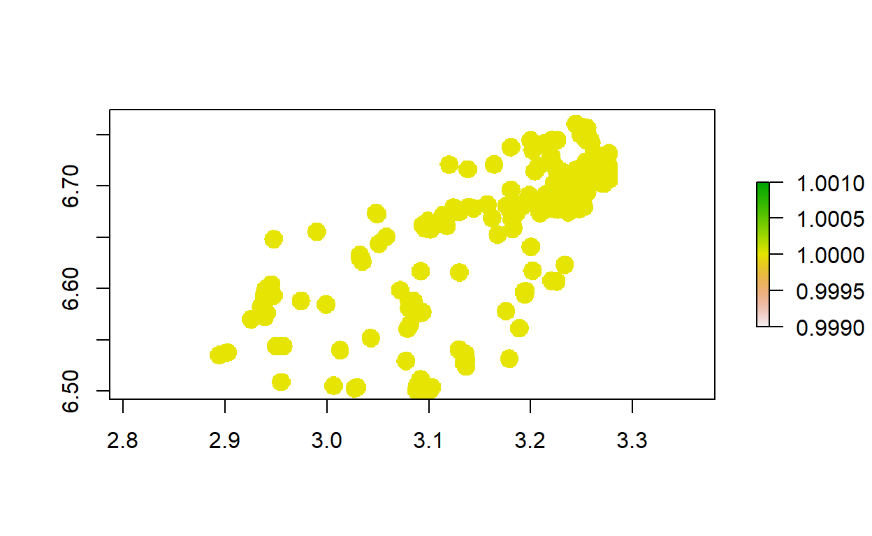
Buffering points ——————————————————–

We want to know how many people are living around each of the health facilities, that leads us to our third spatial manipulation: buffering or drawing a circle of a giving radius around each point.

library(units) # R library to work with unit systems

health_facilities_Ado_buffered <- st_buffer(health_facilities_Ado, dist=set_units(1, km))

We visualise the first observation, that is about the Ado Odo Ii Health Center

health_facilities_Ado[1,]

Simple feature collection with 1 feature and 20 fields
Geometry type: POINT
Dimension:     XY
Bounding box:  xmin: 2.937438 ymin: 6.592648 xmax: 2.937438 ymax: 6.592648
Geodetic CRS:  WGS 84
   FID           editor  timestamp lga_code    lga_name ward_name
1 2835 mokobia.chidinma 2018-12-18    28003 Ado Odo/Ota     Ado 2
  ward_code longitude latitude updated_on accessibil functional
1  OGSADO02  2.937438 6.592648 2019-03-01       <NA> Functional
               category             ownership    type source
1 Primary Health Center Local Government Area Primary   GRID
  alternate_               primary_na
1       <NA> Ado Odo Ii Health Center
                              globalid state_code
1 5e82364d-25dc-4e34-95da-9ea0dbf688ab         OG
                   geometry
1 POINT (2.937438 6.592648)

tm_shape(health_facilities_Ado_buffered[1,])+
  tm_borders()+
  tm_shape(pop_Ado)+
  tm_raster()+
  tm_shape(health_facilities_Ado[1,])+
  tm_dots( size=0.08, id='primary_na', popup.vars=c('category','functional','source'))+
  tm_basemap('OpenStreetMap')

Computing the population ————————————————

We now want to compute the number of people living in 1 km of each facility by aggregating the related grid cells.

health_facilities_Ado_pop <- raster::extract(pop_Ado, health_facilities_Ado_buffered, 
                                             fun=sum, na.rm=T,df=T)

kbl(head(health_facilities_Ado_pop)) %>% 
  kable_minimal()

ID	NGA_population_v2_0_gridded
1	12037.952
2	6758.998
3	7803.548
4	13044.511
5	6647.654
6	3586.548

We see floating point number: this is due to gridded population that has floating point number in its grid cells, as a result of a probabilistic model. It is the most likely value as an average of all the likely values of people count in the grid cell. For more information: WorldPop. 2019. Bottom-up gridded population estimates for Nigeria, version 1.2. WorldPop, University of Southampton. doi:10.5258/SOTON/WP00655.

health_facilities_Ado_buffered$pop <- health_facilities_Ado_pop$NGA_population_v2_0_gridded

EXERCISE: How many people are living in 1km of Ado Odo Ii Health Center?

Click for the solution

health_facilities_Ado_buffered[1,]

Simple feature collection with 1 feature and 21 fields
Geometry type: POLYGON
Dimension:     XY
Bounding box:  xmin: 2.928364 ymin: 6.583597 xmax: 2.946551 ymax: 6.60169
Geodetic CRS:  WGS 84
   FID           editor  timestamp lga_code    lga_name ward_name
1 2835 mokobia.chidinma 2018-12-18    28003 Ado Odo/Ota     Ado 2
  ward_code longitude latitude updated_on accessibil functional
1  OGSADO02  2.937438 6.592648 2019-03-01       <NA> Functional
               category             ownership    type source
1 Primary Health Center Local Government Area Primary   GRID
  alternate_               primary_na
1       <NA> Ado Odo Ii Health Center
                              globalid state_code
1 5e82364d-25dc-4e34-95da-9ea0dbf688ab         OG
                        geometry      pop
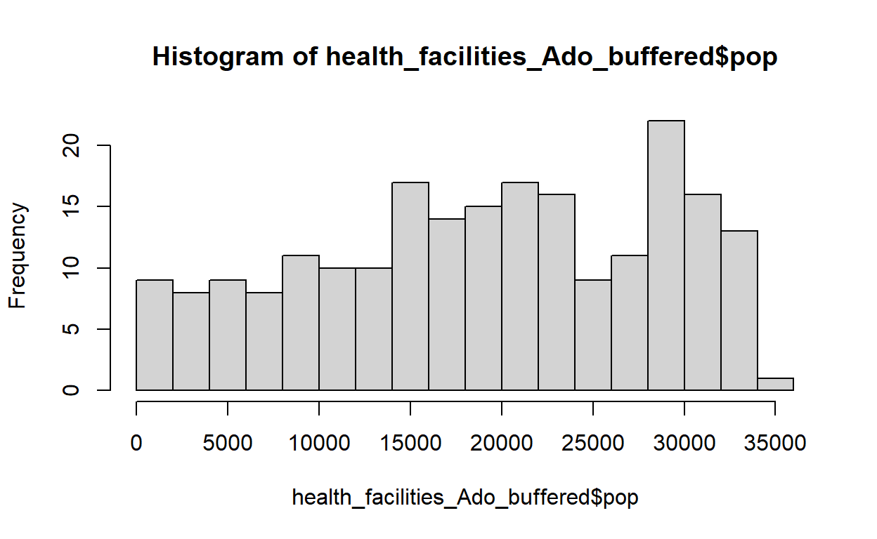
1 POLYGON ((2.937652 6.601684... 12037.95

Let’s look at the distribution of the number of people living at 1km of health facility in Ado.

summary(health_facilities_Ado_buffered$pop)

   Min. 1st Qu.  Median    Mean 3rd Qu.    Max. 
    141   11887   19859   18951   27599   34111 

hist(health_facilities_Ado_buffered$pop, breaks=20)

tm_shape(health_facilities_Ado_buffered)+
  tm_fill('pop', style='pretty', id='pop')+
  tm_shape(health_facilities_Ado)+
  tm_dots( size=0.08, id='primary_na', popup.vars=c('category','functional','source'))+
  tm_basemap('OpenStreetMap')

We can highlight in the less populated area

tm_shape(health_facilities_Ado_buffered %>% 
           filter(pop<1000))+
  tm_fill( id='pop', alpha=0.5, col='grey20')+
  tm_shape(pop_Ado)+
  tm_raster()+
  tm_basemap('OpenStreetMap')

How many people are not covered by health facilities? ——————

We want now to compute the number of people that are not at 1km of a health facility We first need to compute the total number of people at 1km from a health facility. We can’t just sum up the previous column as some people are at less than a 1km of several health facilities such that they will be counted several times.

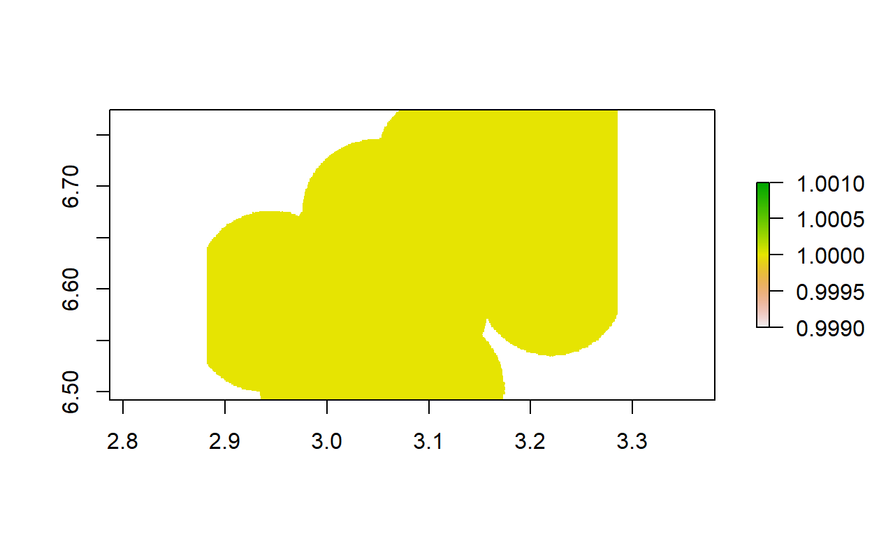
We need a fourth spatial manipulation: rasterizing. We need to convert the buffers into a raster

health_facilities_Ado_buffered_rasterized <- rasterize(health_facilities_Ado_buffered,
                                                       pop_Ado, field=1)
plot(health_facilities_Ado_buffered_rasterized)

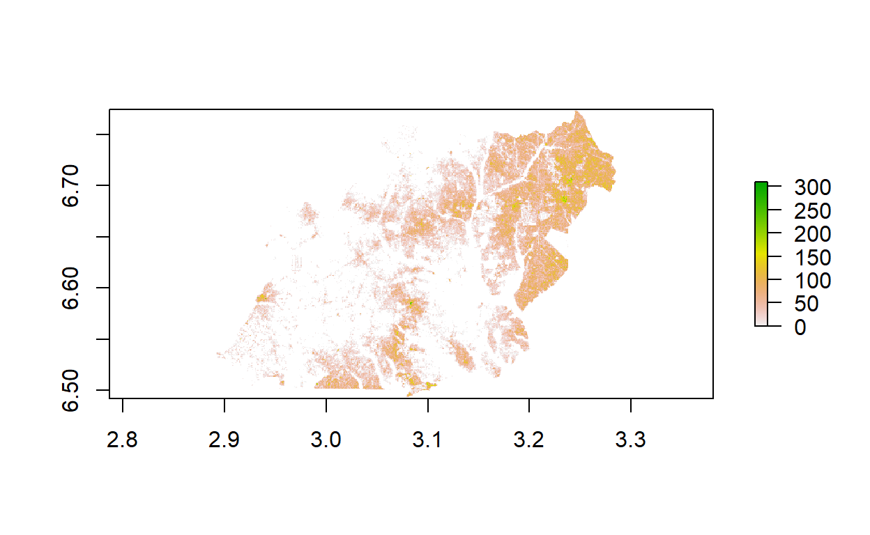
Then we mask the gridded population with the rasterized buffer, which gives us the population covered by the health facilities

pop_Ado_masked <- mask(pop_Ado, health_facilities_Ado_buffered_rasterized)
plot(pop_Ado_masked)

sum(pop_Ado_masked[], na.rm=T)

[1] 1142942

EXERCISE: How many people are not living in a 1km of an health facility? For that purpose we need to compute the number of people living in Ado.

Click for the solution

first method

sum(pop_Ado[], na.rm=T) - sum(pop_Ado_masked[], na.rm=T)

[1] 672583.2

second method

lga_Ado_pop <- raster::extract(pop, lga_Ado, fun=sum, na.rm=T,df=T)
sum(lga_Ado_pop)  - sum(pop_Ado_masked[], na.rm=T)

[1] 672584.2

third method

lga_Ado$mean  - sum(pop_Ado_masked[], na.rm=T)

[1] 672583.2

How many are not covered by a maternity home? —————————

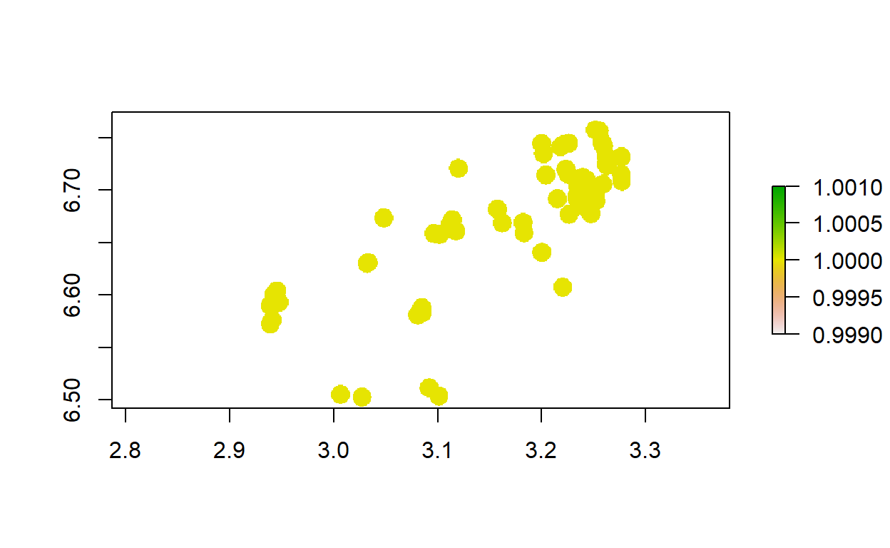
Let’s focused on my health facility type: the maternity homes.

tm_shape(pop_Ado)+
  tm_raster()+
  tm_shape(health_facilities_Ado)+
  tm_dots( size=0.08, id='primary_na', 
           popup.vars=c('category','functional','source'))+
  tm_shape(health_facilities_Ado %>% 
             filter(category=='Maternity Home'))+
  tm_dots(col='darkgreen', size=0.08, id='primary_na', 
          popup.vars=c('category','functional','source'))+
  tm_basemap('OpenStreetMap')

EXERCISE: How many maternity homes are listed in the LGA?

Click for the solution

health_facilities_Ado_buffered_maternity <- health_facilities_Ado_buffered %>% 
  filter(category=='Maternity Home')
nrow(health_facilities_Ado_buffered_maternity)

[1] 69

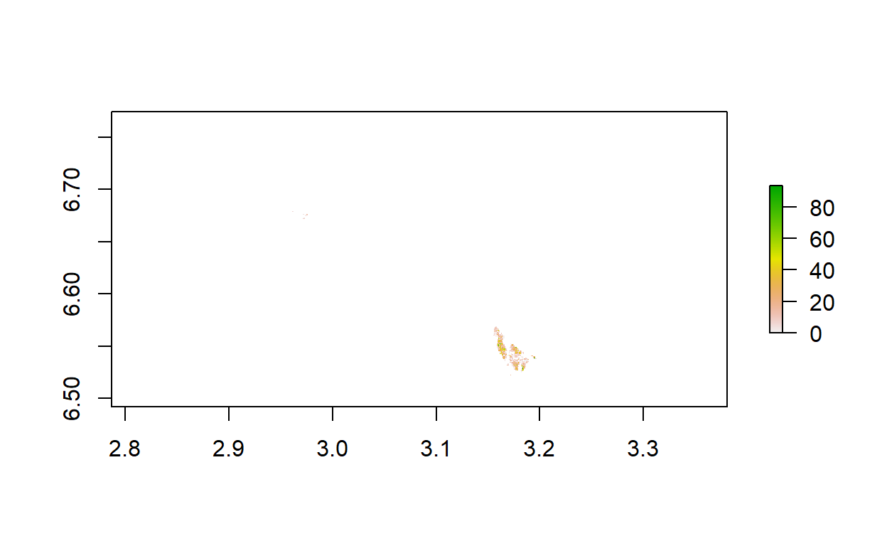
EXERCISE: How many people are not living in a 1km distance of a maternity center?

Click for the solution

health_facilities_Ado_buffered_maternity_rasterized <- rasterize(
  health_facilities_Ado_buffered_maternity, pop_Ado, field=1
)
plot(health_facilities_Ado_buffered_maternity_rasterized)

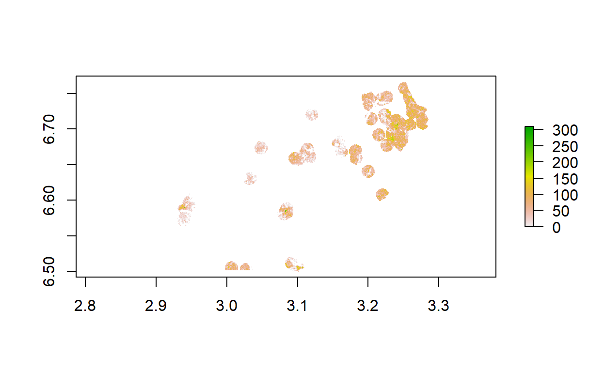
pop_Ado_masked_maternity <- mask(pop_Ado, 
                                 health_facilities_Ado_buffered_maternity_rasterized)
plot(pop_Ado_masked_maternity)

sum(pop_Ado[], na.rm=T) - sum(pop_Ado_masked_maternity[], na.rm=T)

[1] 1149942

What is the furthest a woman has to travel to reach a maternity? ——–

We first subset the maternity homes

health_facilities_Ado_maternity <- health_facilities_Ado %>% 
  filter(category=='Maternity Home')

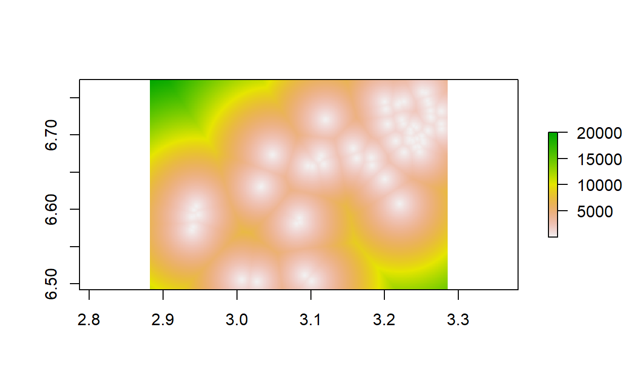
Fifth spatial manipulation: We compute a gridded distance that quantifies the Euclidean distance from each of the grid cells to the nearest maternity

health_facilities_Ado_maternity_distance <- distanceFromPoints(pop_Ado, 
                                                               health_facilities_Ado_maternity)
plot(health_facilities_Ado_maternity_distance)

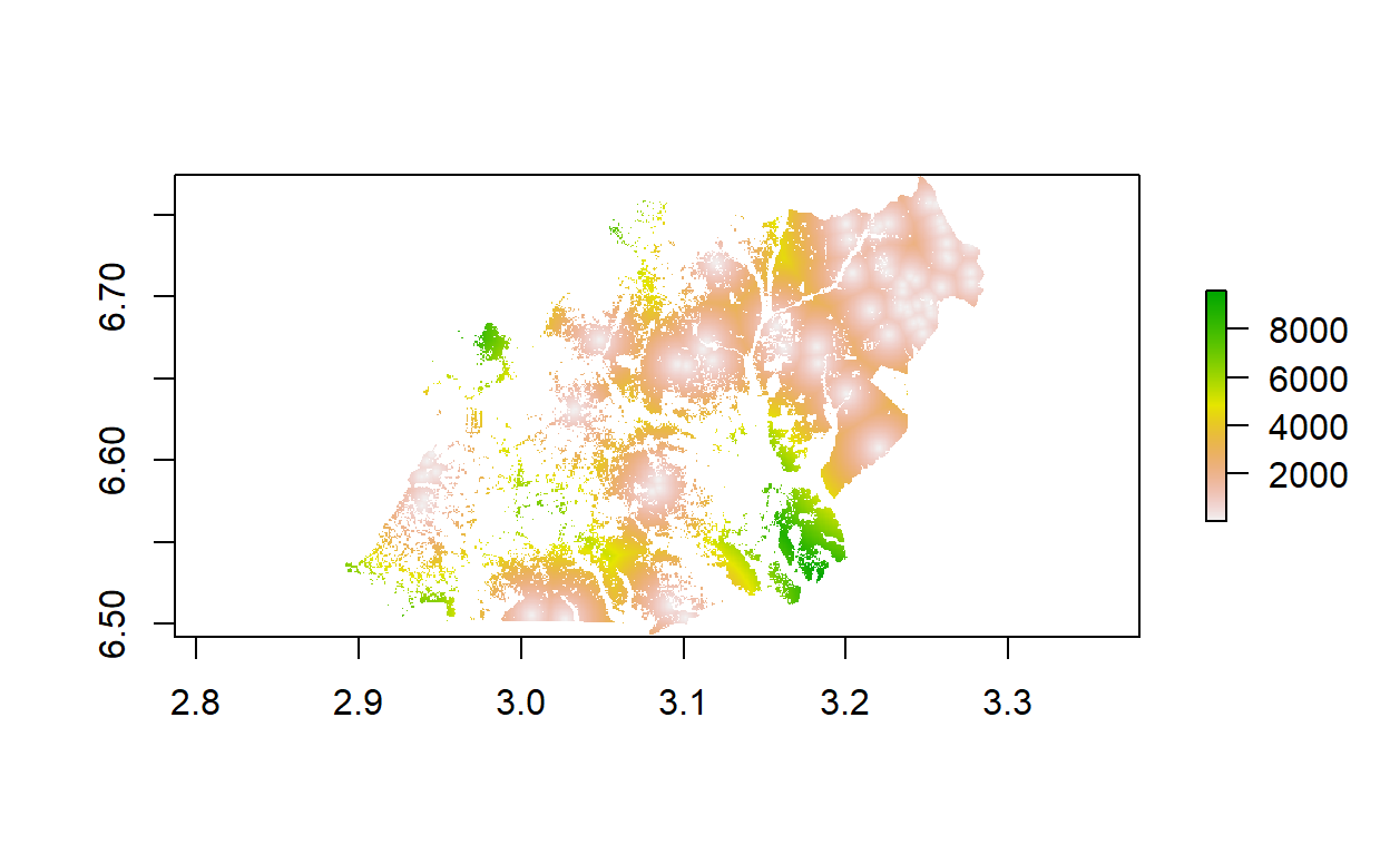
We then focused only on the grid cells that are populated

health_facilities_Ado_maternity_distance_pop <- mask(health_facilities_Ado_maternity_distance, 
                                                     pop_Ado)
plot(health_facilities_Ado_maternity_distance_pop)

We can now have a look at the distribution of the distance to maternity in the LGA.

summary(health_facilities_Ado_maternity_distance_pop[])

   Min. 1st Qu.  Median    Mean 3rd Qu.    Max.    NA's 
  10.68  983.01 1916.11 2369.69 3207.52 9604.39  117769 

EXERCISE: What is the furthest people are leaving from a maternity in Ado?

Click for the solution

max(health_facilities_Ado_maternity_distance_pop[], na.rm=T)

[1] 9604.385

EXERCISE: How many people are living at more than 8km from a maternity? This exercise is based on all the previous analyses steps

Click for the solution

#We compute a buffer of 8 km (rather than 1km)
health_facilities_Ado_maternity_buffered8km <- st_buffer(health_facilities_Ado_maternity,
                                                         dist=set_units(8, km))

#We subtract the population
health_facilities_Ado_maternity_buffered8km_rasterized <- rasterize(
  health_facilities_Ado_maternity_buffered8km, pop_Ado, field=1)
plot(health_facilities_Ado_maternity_buffered8km_rasterized)

pop_Ado_masked_maternity_8km <- mask(pop_Ado, 
                                     health_facilities_Ado_maternity_buffered8km_rasterized, 
                                     inverse=T)
plot(pop_Ado_masked_maternity_8km)

# We sum up the population
sum(pop_Ado_masked_maternity_8km[], na.rm=T)

[1] 9981.121